Tweedie Loss Function
An example: Insurance pricing
A key issue in generating insurance rates is that if premiums are too high, consumers will turn to other companies to purchase insurance. Conversely, if premiums are too low, companies will not earn enough premiums to cover claims.

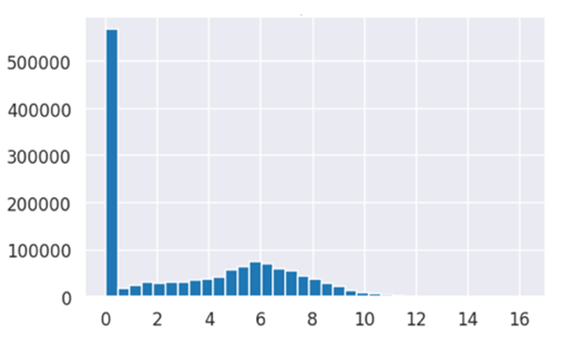
In deciding these rates, therefore, companies need to have an adequate estimation of the expected amount a policyholder might claim in case of an accident. To appropriately set the prices for customers, one crucial task is to predict the size of actual claims. One particular difficulty in predicting such claims is that there are many policyholder’s with no accidents and consequently, no claims. The resulting distribution is therefore positively-skewed, and importantly, is “zero-inflated” with a point mass at 0.

Predicting claim amount
Such zero-inflated distributions may not fare well if loss functions for other (e.g. Gaussian) distributions are used (e.g. RMSE). To deal with this in predictive modelling, one option is to perform the analyses on a subset of the policies, which have at least one claim [1–2]. These might lead to difficulties when generalizing the predictive model to unseen data, which is of course likely to contain many policies with no claims. To adjust for this one could first predict which policies will have at least one claim (e.g. binary classification model) and then separately predict claim size for these policies (e.g. regression model). However, this requires training and regularly updating two separate models which may have different solutions spaces for the same dataset of policies. Alternative approaches have employed Tobit models by treating zero outcomes as censored below some cutoff points [3–4], but these approaches also have disadvantages such as relying on a normality assumption of the latent response.
The “Tweedie” distribution
A Tweedie distribution is a special case of exponential dispersion models and is often used as a distribution for generalized linear models. It can have a cluster of data items at zero and this particular property makes it useful in modelling any zero-inflated dataset such as those regarding insurance claims. Let N be a Poisson random variable, indicating the number of claims a policy has. Furthermore, we can let Zi, (i = 0, 1, 2, …, N) be independent identically distributed Gamma random variables, where Zi indicates the claim amount. We can then define a random variable Z by:

The Tweedie distribution therefore follows a compound Poisson-Gamma distribution, i.e. is a Poisson sum of Gamma random variables. If N=0, then Z=0, thus allowing for a probability mass at zero for policies with no claims. If N>0, then Z is the sum of Ni Gamma random variables, so conditional on N, resulting in a continuous distribution for the positive outcome.
The Tweedie distribution is parametrized by variance power p while φ is an unknown constant. The probability density function (pdf) for a Tweedie distribution on variable y is:

In addition, it is defined for all p values except in the (0,1) interval and has the following distributions as special cases:

Tweedie loss
Because φ is an unknown constant, a(y,φ,p) is also an unknown constant that can be ignored. Based on this Tweedie distribution pdf above, we can use negative log-likelihood to convert the Tweedie distribution to a loss function that will maximize the likelihood of the data given model training:

Estimating the population parameter μ with model predictions, the loss function becomes:

Implementation
The Tweedie loss function can be implemented as a custom loss function in Python:
def tweedie_eval(y_pred, y_true, p=1.5):
   y_true = y_true.get_label()
   a = y_true*np.exp(y_pred, (1-p)) / (1-p)
   b = np.exp(y_pred, (2-p))/(2-p)
   loss = -a + b
   return loss
From the implementation we can see that if y_true = 0, but y_pred > 0, nothing is subtracted and hence the returned loss is larger. Therefore, in order to have the lowest loss possible, both y_true and y_pred must be equal to 0. Deciding on how much to penalize the model for any deviations from this ideal case is controlled by the tweedie variance power parameter p.
Common machine learning packages such as LightGBM and XGBoost support Teedie regression out of the box by using Tweedie loss under the hood, and can be very easily implemented:
xg_reg = xgb.XGBRegressor(objective ='reg:tweedie',
                          tweedie_variance_power=1.5,
                          colsample_bytree = 0.3,
                          learning_rate = 0.1,
                          max_depth = 5, alpha = 10,
                          n_estimators = 10)xg_reg.fit(X_train,y_train)preds = xg_reg.predict(X_test)
Adjusting the ‘tweedie_variance_power’ parameter in the model will result in variable results, so it is best to optimize this for your training (e.g. hyperparameter tuning).
References
[ 1 ] Renshaw, A. E. (1994), “Modelling the Claims Process in the Presence of Covariates,” ASTIN Bulletin, 24, 265–285.
[ 2 ] Haberman, S., and Renshaw, A. E. (1996), “Generalized Linear Models and Actuarial Science,” Statistician, 45, 407–436.
[ 3 ] Van de Ven, W., and van Praag, B. M. (1981), “Risk Aversion and deductibles in Private Health Insurance: Application of an Adjusted Tobit Model to Family Health Care Expenditures,” Health, Economics, and Health Economics, 125–148.
[ 4 ] Showers, V. E., and Shotick, J. A. (1994. “The Effects of Household Characteristics on Demand for Insurance: A Tobit Analysis,” Journal of Risk and Insurance, 61, 492–503.
[ 5 ] Yi Yang, Wei Qian & Hui Zou (2018), “Insurance Premium Prediction via Gradient Tree-Boosted Tweedie Compound Poisson Models”, Journal of Business & Economic Statistics, 36:3, 456–470,
